Voyant Visualizer Guide

View, record, replay, and interact with point clouds from your Carbon 30 sensor.

The Voyant Visualizer is the primary tool for viewing and interacting with point cloud data from your Carbon 30 LiDAR sensor.

Using the Visualizer, you can:

• Stream and record live data from a connected Voyant sensor
• Load and replay recorded point cloud datasets
• Explore 3D point clouds
• Analyze motion, velocity, range, and signal quality

All from a single interface.

---

This guide details the steps to interact with the Voyant Visualizer for live or recorded data.

Note: The Voyant Visualizer replaces Foxglove for most workflows. For ROS users, see the Foxglove Visualization Guide.

Prerequisites

• Completion of the Connection Verification of the Carbon 30 sensor in the Quick Start procedure
• Confirmed access to the Voyant Visualizer, Voyant-provided datasets, and the sensor’s data stream

The following parts of this guide walk you through loading pre-recorded or connecting live data, then interacting with and understanding its point cloud.

1. Data Sources

The Visualizer supports two ways to view data:

1. Playback (Open File): Load a previously recorded point cloud dataset.

2. Live Streaming (Open Connection): Connect directly to a Voyant sensor.

The Data Source panel at the top of the control panel on the left of your screen lets you choose between these options.

1.1. Open File (Playback)

Playback mode allows you to explore previously recorded data.

Click Open File… and select a .bin recording.

You will need a Voyant .bin data file, either:

• Downloaded from available datasets associated with our latest format:
  • car_parking-v0_2_2.bin (720 MB)
  • people_walking-v0_2_2.bin (645 MB)
• Recorded from within the Visualizer.

Use the Playback Controls panel to play, pause, restart, adjust playback rate, loop, and scrub through frames using the progress slider. Note: the Space key can be used to toggle play/pause of data.

1.2. Open Live Connection

Live mode connects directly to a Carbon 30 LiDAR sensor.

Click Open Connection… to connect to a live sensor. See the Verify Connections page for details on establishing a connection to your Carbon 30 sensor.

With a Carbon 30 sensor connected, you should see additional menus for recording and configuring your sensor appear in the Control Panel. The subsequent sections describe how to interact with each.

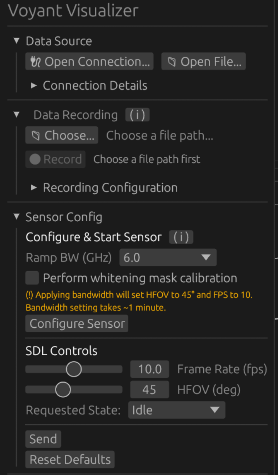
Additional interaction menus available when Carbon 30 sensor is connected.

1.2.1 Configuring SDL Parameters

Your Carbon 30 LiDAR sensor features Software Defined LiDAR (SDL) parameters that allow you to tailor the point cloud’s precision to your needs.

Several customization settings are available to you:

• Ramp BW (GHz) — Set the bandwidth (BW) which controls the balance of distance range precision vs. maximum range.
  • Higher bandwidth = better precision, shorter maximum range
• Perform whitening mask calibration — Toggle on to create a mask to suppress overtly noisy data in the point cloud
  • Note: Calibration takes approximately 10 minutes.

The Configure Sensor initializes the sensor for operation. This button is used to:

• Brings up internal components, like the Carbon 30 laser, after initial boot up
• Applies configuration settings (like those above) Use this button to run the sensor configuration after first powering on the sensor or after changing any SDL parameters.

SDL parameters can be set in the SDL Controls panel, with sliders for:

• Frame Rate (fps) — Sets how many times the sensor scans its field of view per second; more scans = fewer column samples per scan
  • ⇧ FPS = ⇩ column samples per scan = ⇩ azimuthal angular resolution
• HFOV (°) — Sets the Horizontal Field Of View in degrees of the sensor, with a maximum of 120°
  • ⇧ HFOV = ⇧ angular span covered = ⇩ azimuthal angular resolution

These parameters can only be adjusted when the sensor is in an Idle state, set by the Requested State menu.

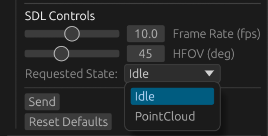
Sensor state selections to adjust and apply SDL parameters.

The Requested State switches the sensor between two modes:

• Idle — Sensor is ready, but not streaming data
• Pointcloud — Sensor is streaming data

The Send button applies the configuration changes (SDL parameter settings) to the sensor.

The standard workflow for parameter adjustment and application is as follows:

1. Adjust SDL Parameters to desired values.

2. Set Requested State to Idle, and click Send

3. Set Requested State to PointCloud, and click Send without touching the sliders again

If successful, you’ll see “Applied” next to the Send button. An error will appear if the combination is invalid. Note: not all SDL parameter combinations are supported.

1.2.2 Recording Live Data

With your Carbon 30 LiDAR sensor connected and streaming data, you can record and save the point cloud over time onto your machine.

To record a dataset:

1. Click Choose… to choose a file path on your machine to place the dataset.

• Choose a folder and title your .bin dataset to be created in the recording.
• Select Save to return to the Voyant Visualizer.
• Note: Your chosen .bin file name will now appear next to the Choose… button.

2. Set file settings and limits with Recording Configuration menu

• Toggle adding a timestamp to your recording file’s name
• Toggle and set Maximum Total limits across all recordings or Per-file limits for each recording for values of:

◦ Number of frames recorded

◦ Duration of recording (s)

◦ File Size (MB)

3. Click the Record button when ready to begin saving frames to a dataset.

• The number of frames captured will be visible and updating live as the dataset is recorded.
• Click the Stop button when satisfied with the capture of your dataset.
• Your recording is now saved to your local machine.

2. Control Panels

This section will walk you through the available options and parameters at your disposal to view and interact with the point cloud from Carbon 30.

2.1. Color Mode

Color modes allow you to visualize different aspects of the point cloud data.

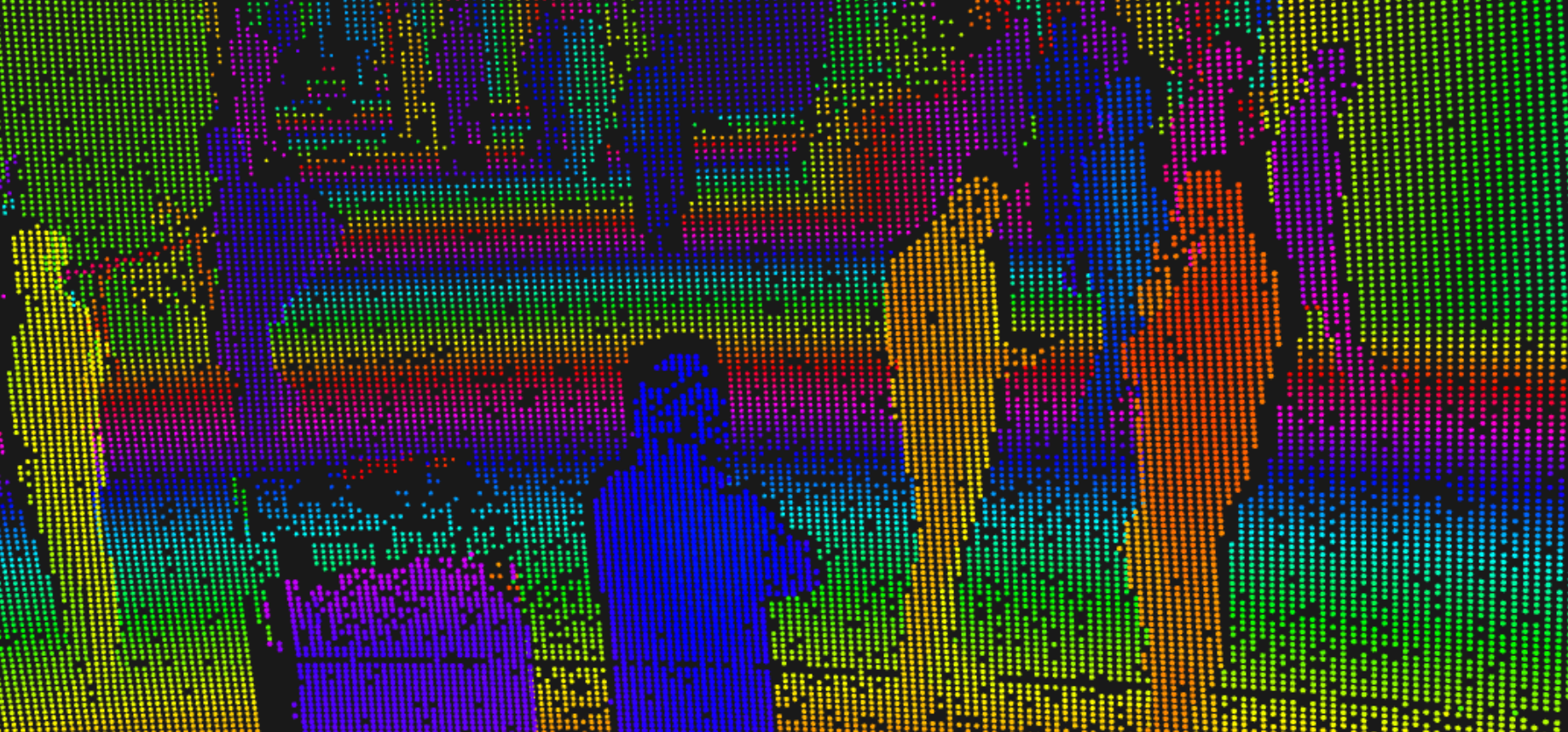
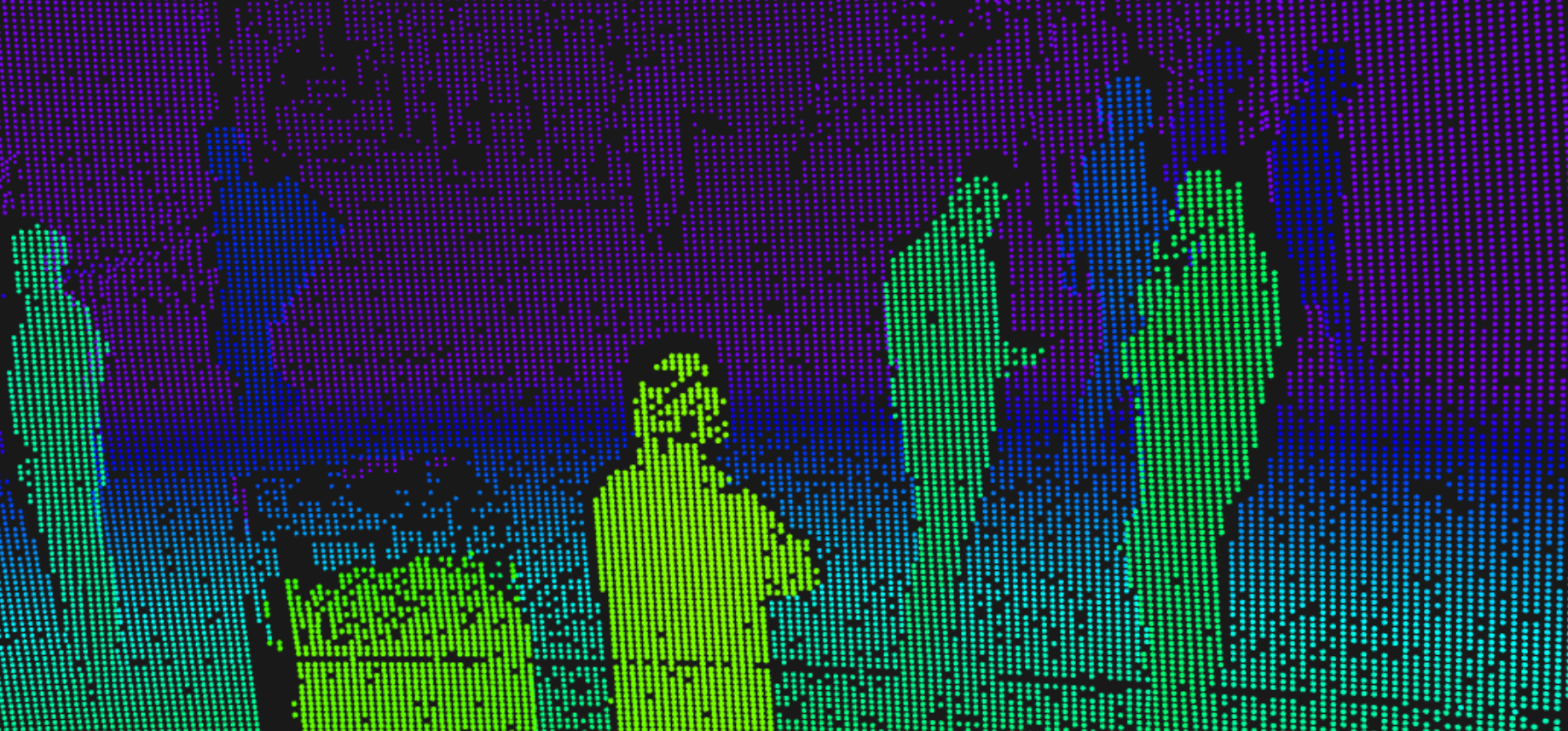
Eight color modes are provided, each highlighting a specific property of the environment. An example of each of the eight colormaps on the same frame of the people_walking-v0_2_2.bin dataset is shown alongside the explanations of each below.

You can switch modes using the dropdown menu or keyboard shortcuts 1–4:

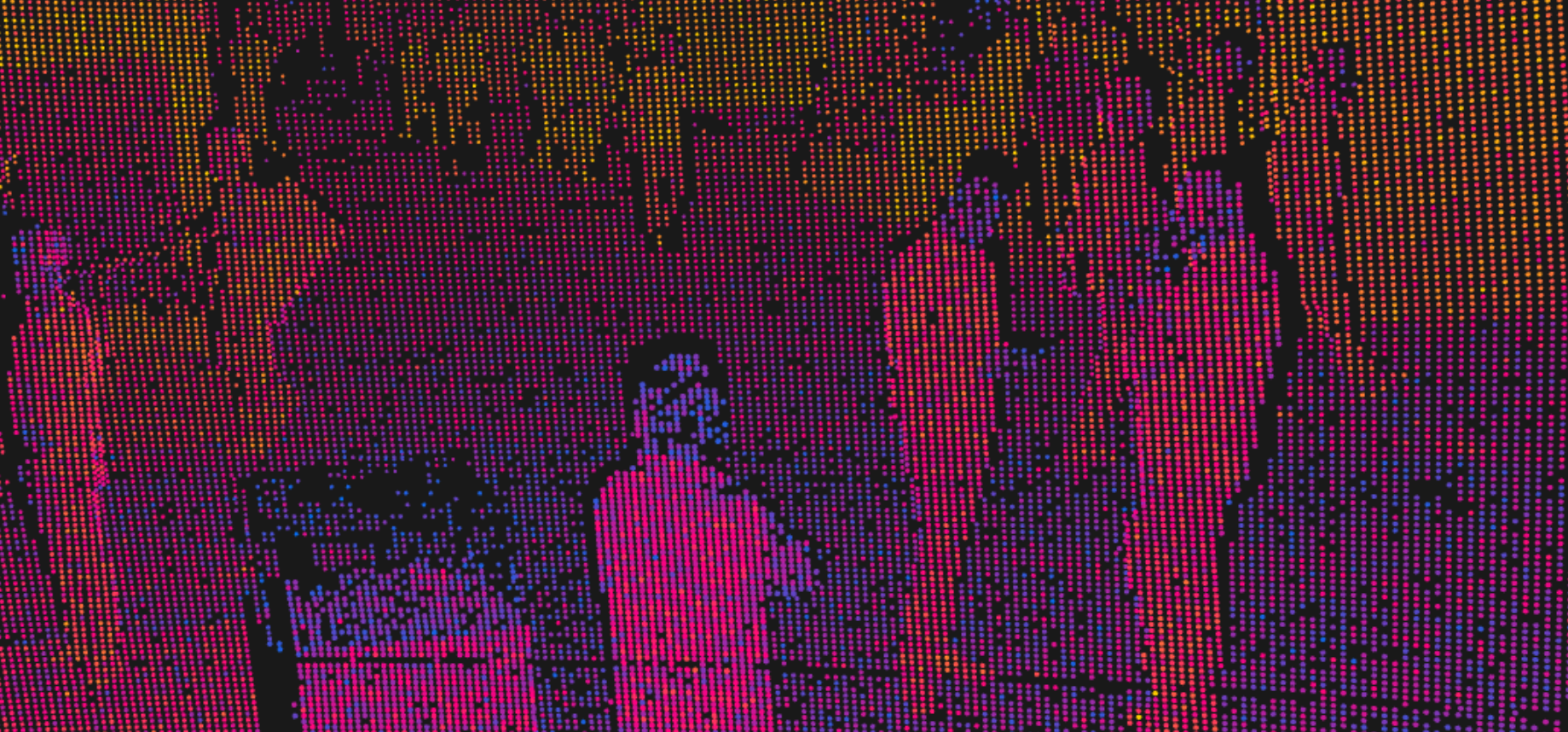
1. Range Bands — Displays distance using repeating HSV color bands.

Associated colorbar

• Helps identify spatial structure and depth
• Adjust band size with your desired distance range with the slider

---

2. Doppler — Displays the radial velocity of objects relative to the sensor

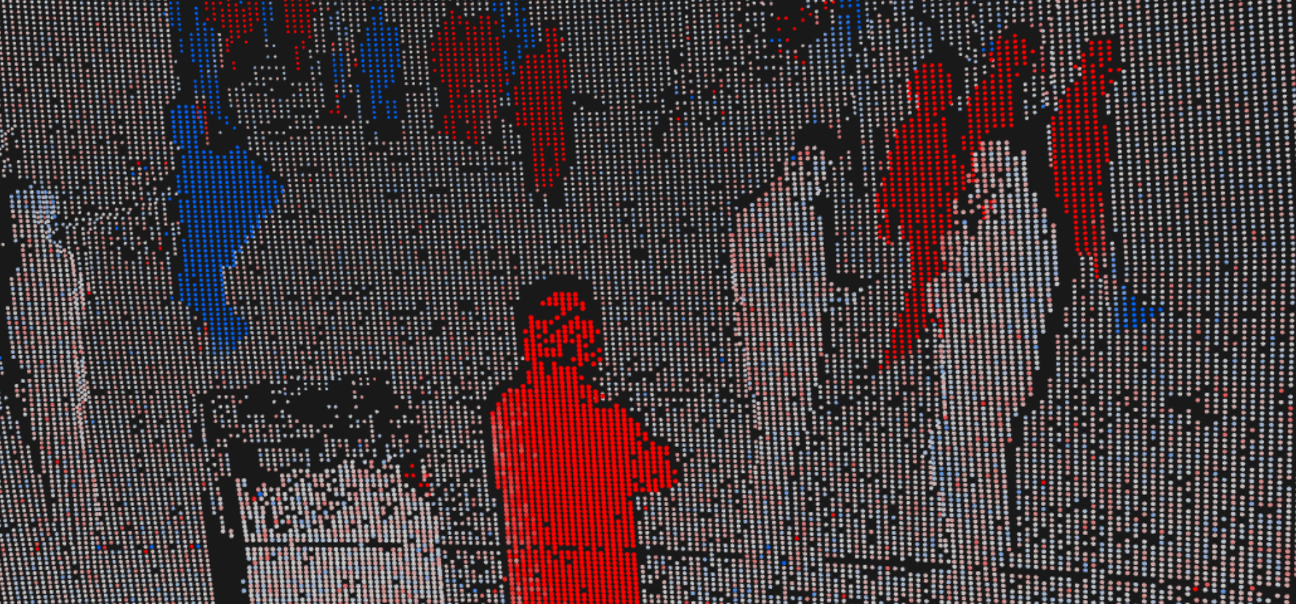
Associated colorbar

• Red — Objects moving away from the sensor (positive radial velocity)
• Blue — Objects moving toward the sensor (negative radial velocity)
• White — Stationary objects (zero radial velocity)
• Use this view to identify moving objects and measure their radial velocity

---

3. SNR — Signal-to-Noise Ratio — Displays signal quality.

Associated colorbar

• "Hotter" colors = higher values = stronger, clearer signal
• "Cooler" colors = lower values = noisier, weaker signals
• Visually identifies data quality and unreliable regions of point cloud

---

4. Reflectance — Displays calibrated reflectance of surfaces

Associated colorbar

• "Hotter" colors = strong reflectance
• "Cooler" colors = weak reflectance
• Visually identifies materials with different surface properties

---

Additional modes (no keyboard shortcuts):

• X/Y/Z — Displays spatial coordinate values along each axis

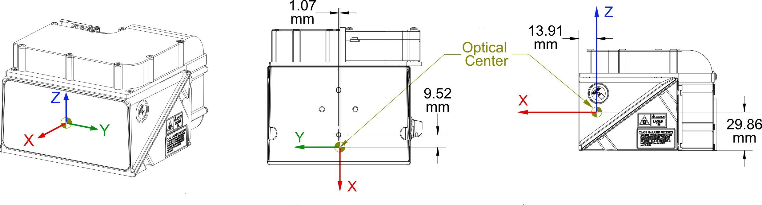
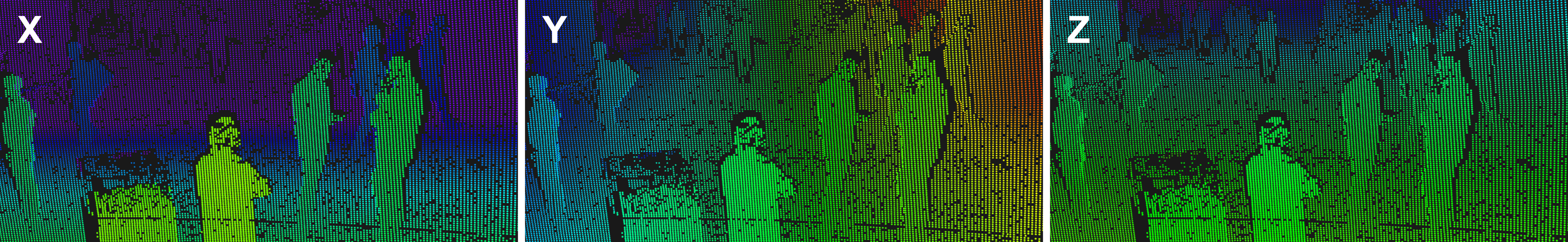
Associated colorbar

• X — forward/back
• Y — left/right
• Z — height
• Use to understand orientation and coordinate alignment of the point cloud

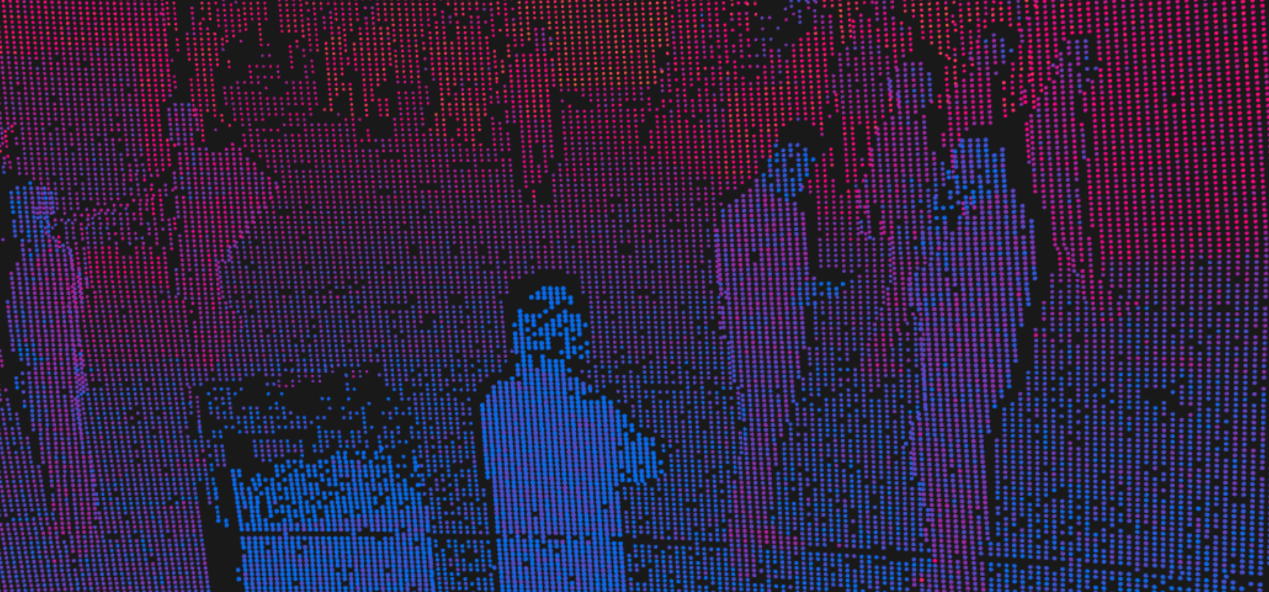
• Range (min/max) — Displays absolute distance from the sensor

Associated colorbar

• Continuous gradient (no repeating like in Range Bands mode) between nearest and farthest data points
• Identifies distances between objects clearly

2.2. Rendering

• Use the Point Size (mm) slider to control the visibility of points in the point cloud.
• Set Point Quality to set the roundness of the points in the point cloud.
  • Scales roundness up from Square → Low → Medium → High
  • Lower quality reduces compute load if you experience performance issues.
• Toggle Mirror Mode with M to horizontally flip data (about the y-axis).
• Toggle Range Compensated Point Size with the adjustable scale factor to normalize the visibility of near and far points in the point cloud.
  • Toggling on makes the data points look more visually consistent across the point cloud. When off, the points farther from the sensor appear smaller as the point cloud becomes less dense.

2.3. Scene Elements

• Toggle origin and axes visibility with Show Axes
  • Use the Axes Length (m) slider to set the length the axes extend from the origin.
• Toggle origin and radially spaced rings visibility with Range Rings
  • Preset defines preconfigured spacing of the range rings with options:
    • Auto — Rings at [0.5, 1, 5, 10, 25, 50, 100, 200] m
    • Short Range — Rings at [0.5, 1, 2, 5, 10, 25] m
    • Medium Range — Rings at [5, 10, 25, 50, 100] m
    • Long Range — Rings at [10, 50, 100, 200] m
    • Custom — Rings at spacing of your choosing set with adjustable sliders on Spacing (m) and Max (m) distance bound
  • Adjust Label Size (m) on each range ring with the slider.

2.4. Camera

• View of the LiDAR point cloud using preset orientations: Rear Elevated (Default), Rear, Top-Down, Left, Right, Front
• Manipulate the view directly using the mouse.
  • Left Mouse — Orbit = rotate around the point cloud
  • Right Mouse — Pan = move left/right relative to the current view
  • Scroll — Zoom = move closer to/farther away from the current view point
• Reset the view to the selected orientation by pressing the Reset Camera Position button or the C key

3. Details

3.1. Frame Info

The Frame Info panel displays metadata for the current frame:

• Frame Index — Numerical position of the current frame in the stream or file
• Timestamp — Time of capture
• Point Count — Number of valid points in the current frame
  • Invalid points (points deemed too noisy to be a true return) are automatically filtered out
• Point Cloud FPS — Incoming frame rate from the sensor or playback
• Points Per Second — Number of points in the point cloud per second

3.2. Help (Controls)

Keyboard shortcuts for all controls are listed in the Help (Controls) panel at the bottom of the sidebar.